Validation¶

Even if the core of the pyTAMS algorithm is not particularly complex, details of the implementation can lead to systematic biases on the rare event probability estimator, especially when the event $\mathcal{E}$ probability becomes very rare ($P(\mathcal{E}) < 10^{-6}$).

In this section we validate pyTAMS implementation on a couple of simple, low dimensional cases and since the algorithm is decoupled from the physics of the model, the validity extends to more complex physics model for which no theoretical data is available.

1D Ornstein-Uhlenbeck process¶

The simple case of a one dimensional Ornstein-Uhlenbeck (OU) process is part of pyTAMS examples suite. It is an interesting case to consider since Lestang et al. used this model while developing the TAMS algorithm. In contrast with the Theory Section, the OU process does not feature multistability, but we are interested in predicting the occurrence of extreme values of the process.

Before jumping into TAMS results, we can provide an estimate of the process stationary distribution $P_s(x)$ using a very long trajectory ($10^{8} steps$). The OU process parameters are set to $\theta = 1.0$ and $\epsilon = 0.5$, for which theoretical $P_s(x) = \mathcal{N}(0,\sigma)$ with $\sigma = \sqrt{\epsilon/\theta}$. The log-scale plot of the distribution shows that extreme values of the process ($abs(x) > 4\sigma$) are poorly sampled using such a Monte Carlo approach.

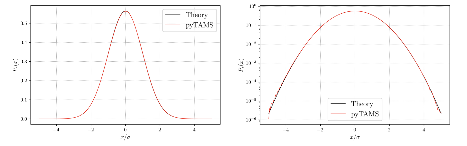
_images/distribution_OU1D.png — Figure 4 :Stationary distribution $P_s(x)$ of the OU process obtained with TAMS¶

We will now use TAMS to predict the return time $r(a)$ of the value $a$ in the OU process. This is specifically what TAMS was developed for. The results of TAMS are obtained from 25 independent TAMS runs, with $N = 100$, $T_a = 5 \tau_c$ and $\xi_{max} = 8\sigma$. The long trajectory used in producing Figure 4 is processed using the block-maximum method to provide an estimate of $\hat{r}(a)$ and the theoretical $r(a)$ in also given by equation A6 of Lestang et al.. The graph Figure 5 shows the return time in abscissa and the value of $a$ in ordonate for all three methods. The agreements between pyTAMS and the theoretical value of the return time demonstrate that the current implementation is able to correctly estimate rare events, down to very probability ($P(\mathcal{E}) < 10^{-10}$)

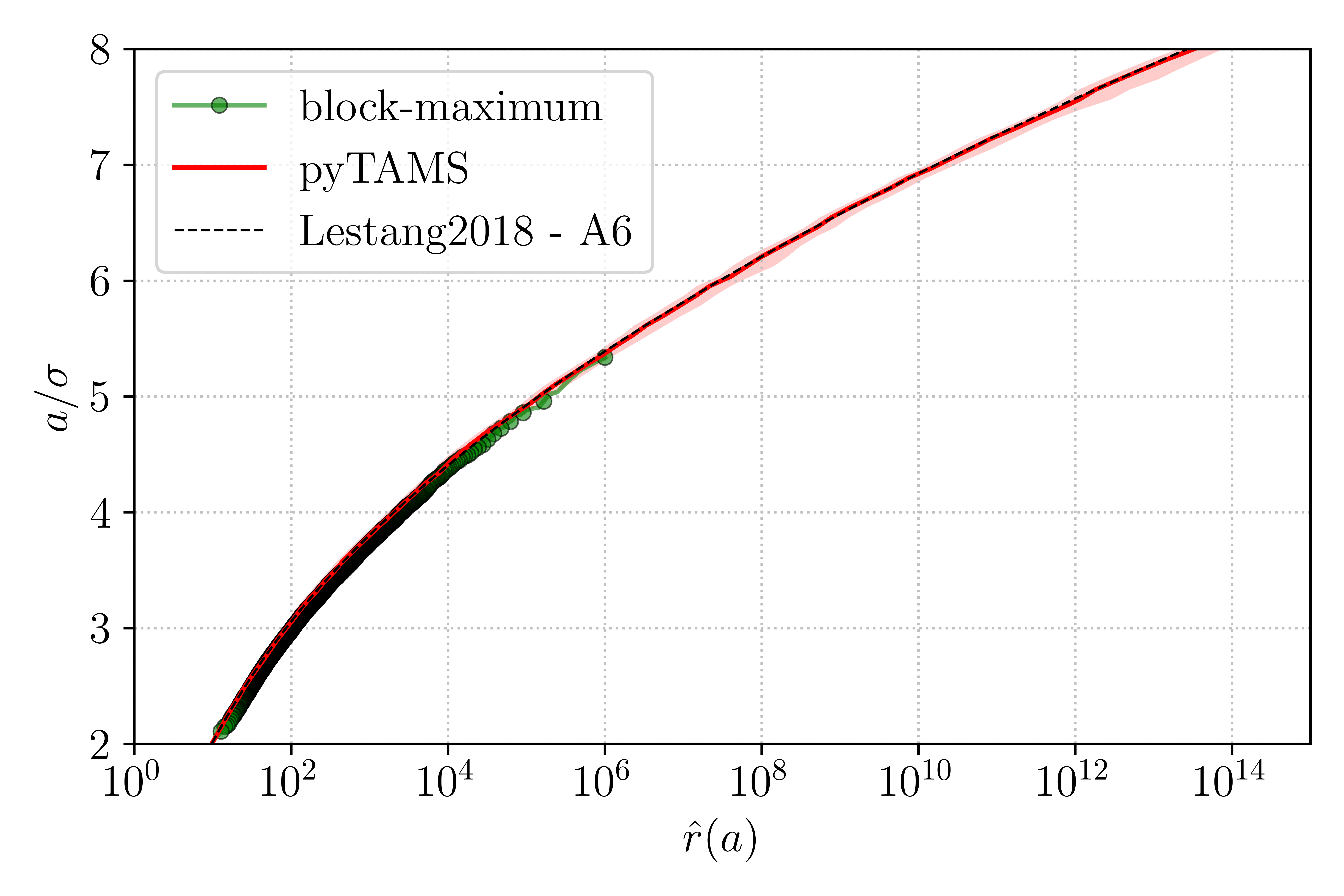
_images/returntimes_OU.png — Figure 5 : Comparison of return times $\hat{r}(a)$ of an OU process obtained with the block-maximum method, TAMS and the theoretical expression of Lestang et al.¶

2D double well case¶

The case of the 2 dimensional double well (readily available in pyTAMS examples) has been extensively studied by Baars and we will use Baars data as reference for pyTAMS results.

Specifically, let’s look at the transition probability from one well to the other within a time horizon $T_a$ decreasing from 10 to 2 time units. We will run TAMS with a small ensemble $N = 50$, iterating until all the ensemble members reach $\mathcal{B}$, the well located at $X_t = x_B = (1.0, 0.0)$. At each value of $T_a$, we run $K = 100$ independent runs of TAMS to compute the transition probability estimate:

\[\overline{P}_K = \frac{1}{K}\sum_{k=1}^K \hat{P}_k\]

where $\hat{P}_k$ is the transition probability of a single TAMS run. Note that Baars used $N=10000$ and $K = 1000$ which provides a more accurate estimator. Following Baars, we also use the 25-75 interquartile range (IQR) to give an indication of the estimator quality (standard confidence interval are not appropriate for near-zero distributions).

Figure 6 shows pyTAMS $\overline{P}_K$ in the range of values of $T_a$ considered, along with the IQR given by the shaded area and results from Baars.

_images/valid_doublewell2D.png — Figure 6 : Transition probability estimate $\overline{P}_K$ at several values of $T_a$ in the 2D double well case¶

The agreement between the two datasets is good, even though the accuracy of the pyTAMS results are expected to be lower due to the relatively small $N$ and $K$ used compared to Baars. As $T_a$ decreases, the IQR become less symmetric around $\overline{P}_K$, mostly due to the choice of a static score function which causes TAMS to stall if the transition is initiated too close to $T_a$.