Theory
Stochastic dynamical systems
Stochastic dynamical systems describe the evolution of a random process \((X_t)_{t \ge 0}\), where the state \(X_t \in \mathbb{R}^{d}\) evolves according to probabilistic rules rather than deterministic dynamics only. If the system is Markovian, i.e. \(X_{t+\Delta t}\) depends only on the current state \(X_t\), its behavior can be characterized by a stochastic differential equation (SDE) of the form:
where \(f : \mathbb{R}^{d} \to \mathbb{R}^{d}\) denotes the drift term, governing the deterministic component of the dynamics, while \(g : \mathbb{R}^{d} \to \mathbb{R}^{d \times m}\) represents the diffusion matrix, which scales the stochastic forcing introduced by the \(m\)-dimensional Wiener process \(W_t \in \mathbb{R}^{m}\).
Solving analytically the above SDE to obtain the system probability distributions is rarely feasible, especially in nonlinear or high-dimensional settings. Markov chain Monte Carlo (MCMC) methods address this challenge by constructing a discrete-time Markov chain whose stationary distribution approximates the target distribution of the stochastic dynamical system. In this context, MCMC produces an ensemble of sample trajectories \(\{X_t^{(k)}\}_{k=1}^K\), where each \(X_t^{(k)}\) represents the \(k\)-th simulated path of the underlying Markov process. These sampled trajectories allow to approximate expectations \(\mathbb{E}[h(X_t)]\), estimate uncertainty, and analyze long-term behavior even when closed-form expressions for the dynamics are inaccessible.
Rare events
Rare events of the above stochastic dynamical system correspond to outcomes of the process \(X_t\) that occur with very low probability but often carry significant impact, such as extreme fluctuations in financial markets, system failures, climate extremes or transitions between metastable states in physical systems. Let denote such a rare event by
where \(\mathcal{C}\) is a subset of the state space \(\mathbb{R}^{d}\) with small probability under the distribution of \(X_t\). Quantities of interest often involve the expectation of an indicator function
Estimating \(\mathbb{P}(\mathcal{E})\) using plain Monte Carlo involves drawing \(K\) independent trajectories \(\{X_t^{(k)}\}_{k=1}^K\) and computing the empirical average, resulting in an estimator:
While unbiased, this estimator suffers from a severe relative error issue when the occurrence of the event \(\mathcal{E}\) is rare. Specifically, the relative error writes (Rubino and Tuffin):
which implies that achieving a fixed relative accuracy requires \(K = \mathcal{O}(1 / \mathbb{P}(\mathcal{E}))\) samples. For rare events where \(\mathbb{P}(\mathcal{E})\) is extremely small, this makes plain Monte Carlo computationally infeasible, motivating the use of variance reduction and specialized rare-event sampling techniques such as importance sampling, splitting, or rare-event-focused Markov chain Monte Carlo methods.
Trajectory-adaptive multilevel sampling
Trajectory-Adaptive Multilevel Sampling TAMS (Lestang et al.) is a rare event technique of the Importance Splitting (IS) family, derived from Adaptive Multilevel Sampling (AMS) (see for instance the perspective on AMS by Cerou et al.). AMS (Cerou and Guyader) was designed with transition between metastable states in mind. Using the previously introduced notations, let’s define a state \(\mathcal{A}\), a subset of \(\mathbb{R}^{d}\), and the associated return time to \(\mathcal{A}\):
for a Markov chain initiated at \(X_t(t=0) = X_0 = x_0 \notin \mathcal{A}\). Let’s define similarly \(\tau_{\mathcal{B}}\) for a state \(\mathcal{B}\). Both \(\mathcal{A}\) and \(\mathcal{B}\) are metastable regions of the system phase space if a Markov chain started in the vicinity of \(\mathcal{A}\) (resp. \(\mathcal{B}\)) remains close to \(\mathcal{A}\) (resp. \(\mathcal{B}\)) for a long time before exiting. AMS aims at sampling rare transition events \(E_{\mathcal{A}\mathcal{B}}\) between \(\mathcal{A}\) and \(\mathcal{B}\)
for initial conditions \(x_0\) close to \(\mathcal{A}\). Such transitions are rare owing to the attractive nature of the two metastable regions. The idea of multilevel splitting is to decompose this rare event into a series of less rare events by defining successive regions \(\mathcal{C}_i\):
and \(E_{\mathcal{A}\mathcal{C}_i}\) the event \(\tau_{\mathcal{C}_i} < \tau_{\mathcal{A}}\). Using the conditional probabilities \(p_i = \mathbb{P}(E_{\mathcal{A}\mathcal{C}_i} | E_{\mathcal{A}\mathcal{C}_{i-1}})\) for \(i > 1\), we have:
In practice, the definition of the regions in the state phase space \(\mathbb{R}^{d}\) relies on system observables, \(\mathcal{O}(X_t)\). These observables can be combined into a score function \(\xi(X_t) : \mathbb{R}^{d} \to \mathbb{R}\) mapping your high dimensional state space to a more manageable one dimensional space. The \(\mathcal{A}\) and \(\mathcal{B}\) states can then be defined using \(\xi(X_t)\):
The successive regions \(\mathcal{C}_i\) can similarly be defined using levels of \(\xi\) between \(\xi_a\) and \(\xi_b\). In AMS, these levels are automatically selected by the algorithm which alleviate a strong convergence issue arising with older multilevel splitting methods which required selecting these levels a-priori, using the practitioner intuition.
In addition, TAMS targets the evaluation of \(\mathcal{A}\) to \(\mathcal{B}\) transitions within a finite time interval of the Markov chain \([0, T_a]\), which then requires the use of a time dependent score function \(\xi(X_t,t)\).
TAMS algorithm
The idea behind (T)AMS is to iterate over a small ensemble of size \(N\) of Markov chain trajectories (i.e. much smaller than the number of trajectories needed for a reliable sampling of the rare transition event with Monte Carlo), discarding trajectories that drift away from \(\mathcal{B}\), while cloning/branching trajectories that are going towards \(\mathcal{B}\). This effectively biases the ensemble toward the rare transition event.
The selection process uses the score function \(\xi(X_t,t)\). At each iteration \(j\) of the algorithm, the trajectories are ranked based on the maximum of \(\xi(X_t,t)\) over the time interval \([0, T_a]\):
for \(tr \in [1, N]\). At each iteration, the \(l_j\) trajectories with the smallest value of \(\mathcal{Q}\), \(min (\mathcal{Q}_{tr}) = \mathcal{Q}^*\), are discarded and new trajectories are branched from the remaining trajectories and advanced in time until they reach \(\mathcal{B}\) or until the maximum time \(T_a\) is reached. The process is illustrated on a small ensemble in the following figure:
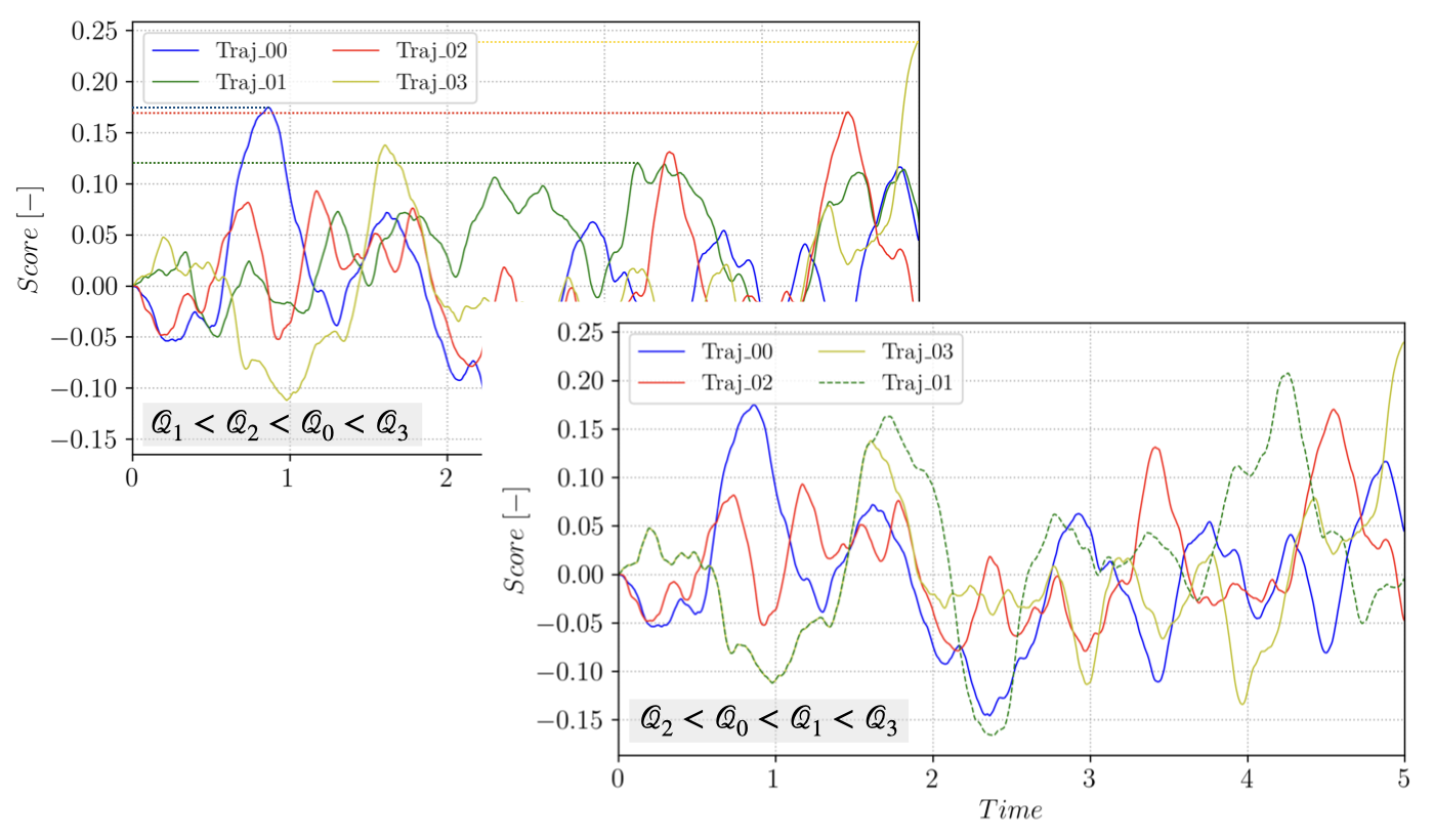
Figure 1 Branching trajectory \(1\) from \(3\), starting after \(\xi(X_3(t),t) > \mathcal{Q}^*\).
Note that at each iteration, selecting \(\mathcal{Q}^*\) and discarding the \(l_j\) lowest trajectories amounts to defining a new \(\mathcal{C}_i\) and defining \(p_i = 1 - l_j/N\).
For each cloning/branching event, a trajectory \(\mathcal{T}_{rep}\) to branch from is selected randomly (uniformly) in the \(N-l_j\) remaining trajectories in the ensemble. The branching time \(t_b\) along \(\mathcal{T}_{rep}\) is selected to ensure that the branched trajectory has a score function strictly higher that the discarded one:
This iterative process is repeated until all trajectories reached the measurable set \(\mathcal{B}\) or until a maximum number of iterations \(J\) is reached. TAMS associate to the trajectories forming the ensemble at step \(j\) a weight \(w_j\):
Note that \(w_0 = 1\). The final estimate of \(p\) is given by:
where \(N_{\in \mathcal{B}}^J\) is the number of trajectories that reached \(\mathcal{B}\) at step \(J\).
TAMS only provides an estimate of \(p\) and the algorithm is repeated several times in order to get a more accurate estimate, as well as a confidence interval. The choice of \(\xi\) is critical for the performance of the algorithm as well as the quality of the estimator. Repeating the algorithm \(K\) time (i.e. performing \(K\) TAMS runs) yields:
Theoretical analysis of the AMS method (which also extends to TAMS) have showed that the relative error of \(\overline{P}_K\) scales in the best case scenario:
while the worst case scenario is similar to plain Monte Carlo:
The best case scenario corresponds to the ideal case where the intermediate conditional probabilities \(p_i\) are perfectly compute, which corresponds to using the optimal score function \(\overline{\xi}(y) = \mathbb{P}_y(\tau_{\mathcal{B}} < \tau_{\mathcal{A}})\), also known as the commitor function. One will note that the commitor function is precisely what the TAMS algorithm is after for \(y = X_0 = x_0\).
An overview of the algorithm is provided hereafter:
Simulate \(N\) independent trajectories of the dynamical system between [0, \(T_a\)]
Set \(j = 0\) and \(w[0] = 1\)
while \(j < J\):
compute \(\mathcal{Q}_{tr}\) for all \(tr \in [1, N]\) and sort
select the \(l_j\) smallest trajectories
for \(i \ in [1, l_j]\):
select a trajectory \(\mathcal{T}_{rep}\) at random in the \(N-l_j\) remaining trajectories
branch from \(\mathcal{T}_{rep}\) at time \(t_b\) and advance \(\mathcal{T}_{i}\) until it reaches \(\mathcal{B}\) or \(T_a\)
set \(w[j] = (1 - l_j/N) \times w[j-1]\)
set \(j = j+1\)
if \(\mathcal{Q}_{tr} > \xi_{b}\) for all \(tr \in [1, N]\):
break
Simple 1D double well
To illustrate the above theory on a simple example, we now consider the concrete case of a 1D double well stochastic dynamical system described by:
where \(f(X_t) = - \nabla V(X_t)\) is derived from a symmetric potential:
\(\epsilon\) is a noise scaling parameter, and \(W_t\) a 1D Wiener process.
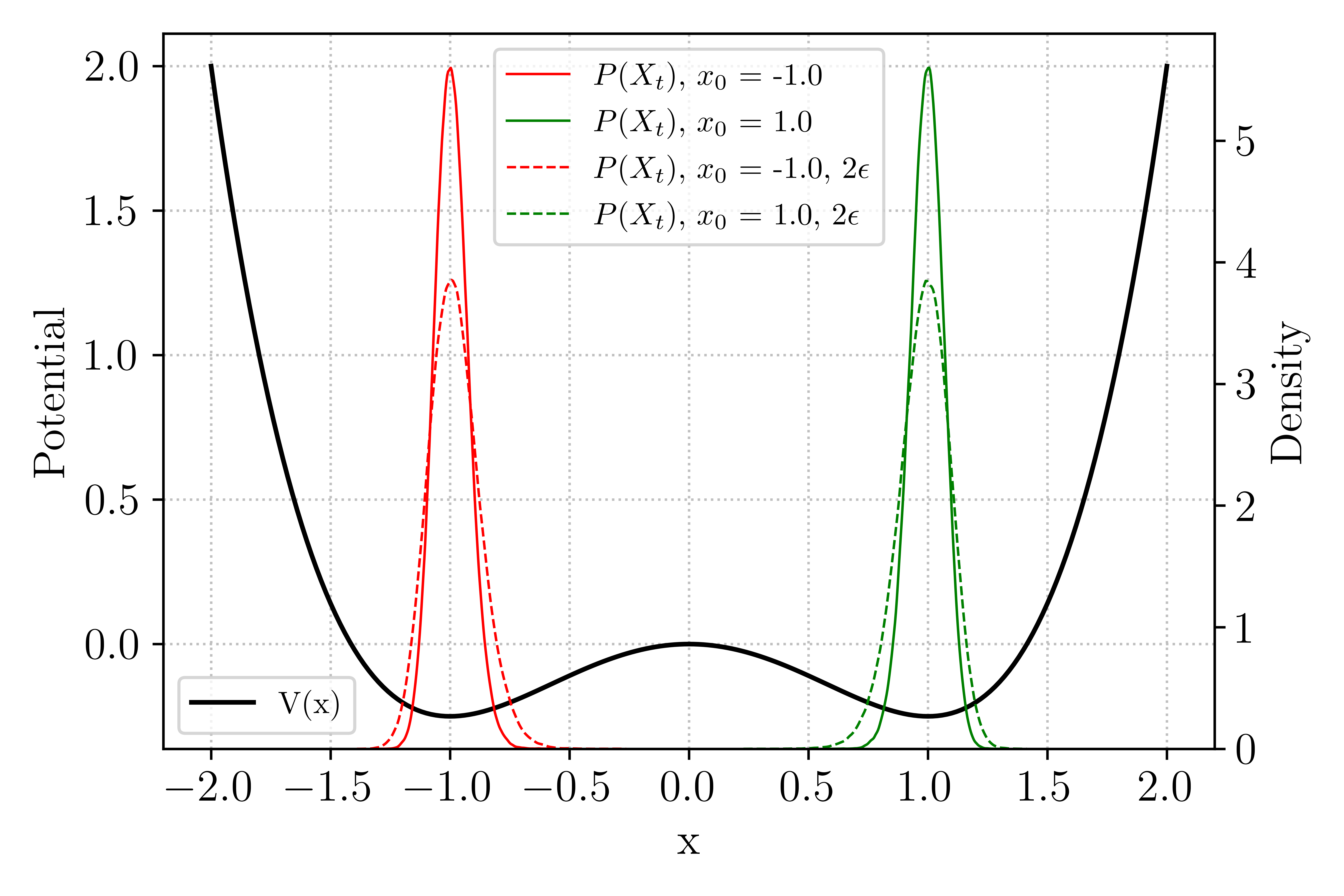
Figure 2 1D double well, showing the potential \(V\) and distribution function of long Markov chains starting in each well, at two noise levels.
The figure above shows the two metastable states of the model: for long Markov chains (\(T_f = N_t \delta_t\) with \(N_t = 1e^6\) and \(\delta_t = 0.01\)) initiated in either of the two well (clearly marked by local minima of the potential \(V(x)\)), the model state distributions \(P(X_t)\) remains in the well, with the distribution widening as the noise level is increased.
Using TAMS, we want to evaluate the transition probability from \(\mathcal{A}\), the well centered at \(x_{\mathcal{A}} = -1.0\), to \(\mathcal{B}\) the well centered at \(x_{\mathcal{B}} = 1.0\), with a time horizon \(T_a = 10.0\) and setting \(\epsilon = 0.025\).
Even for a simple system like this one, there are multiple possible choices for the score function. We will use a normalized distance to \(\mathcal{B}\):
and select \(\xi_b = 0.95\). Note that in this case, choosing a fixed value of \(\xi_a\) is possible but for simplicity, all the trajectories are initialized exactly at \(X_0 = x_{\mathcal{A}}\). Additionally, no dependence on time is included in the score function (it is referred to as a static score function). The animation below shows the evolution of the TAMS trajectories ensemble (each trajectory \(\xi(X_t)\) as function of time is plotted), during the course of the algorithm. As iterations progress, the ensemble deviates from the system metastable state near \(\xi(X_t) = 0\) towards higher values of \(\xi(X_t)\).
Figure 3 Evolution of the TAMS trajectories ensemble (\(N = 100\), \(l_j = 1\)) over the course the algorithm iterations.
Eventually, all the trajectories transition to \(\mathcal{B}\) and the algorithm stops. The algorithm then provides \(\hat{P} = 4.2e^{-5}\). As mentioned above, the algorithm will need to be performed multiple times in order to provide the expectancy of the estimator \(\hat{P}\), and comparing the relative error to the lower and upper bound mentioned above can be used to evaluate the quality of the employed score function.