Tutorials

This set of tutorials is designed to guide the users through the process of encapsulating their stochastic dynamical system into the framework of pyREVS in order to smoothly leverage the capabilities of rare event techniques.

With the exception of a few example cases shipped with the code, pyREVS will always require the user to formulate her/his problem in as little as a few dozens of lines of code, to hundreds if the complexity of the model warrants it.

1D double well

In this first tutorial, our aim is to implement the 1D double well model already presented at the end of the Theory Section. This model is not provided out-of-the-box in pyREVS and will be written from scratch.

Background

As a reminder, the 1D double well stochastic dynamical system can be described with the following stochastic differential equation:

\[dX_t = f(X_t)\,dt + \sqrt{2\epsilon}\,dW_t.\]

where \(f(X_t) = - \nabla V(X_t)\) is derived from a symmetric potential:

\[V(x) = \frac{1}{4}x^4 - \frac{1}{2}x^2,\]

\(X_t \in \mathbb{R}\) is our Markov process, \(\epsilon\) is the noise scaling parameter and \(dW_t\) a 1D Wiener process. A simple Euler-Maruyama method to advance the system in time. In this tutorial, we will try Monte-Carlo, TAMS as well as AMS sampling strategies.

Getting set up

If you haven’t done so yet, let’s get the latest version of pyREVS installed on your system. In your favorite environment manager, simply use:

pip install pyrevs
tams_check

The second line check that pyREVS is effectively installed and should return (with proper version numbers):

== pyREVS vX.Y.Z :: a rare-event finder tool ==

Now create a new folder for us to work in:

mkdir pyrevs_1d_doublewell
cd pyrevs_1d_doublewell

Writing the forward model

Our first task is to implement the SDE provided above in a class that can interact with pyREVS. As mentioned in the Implementation Section, one needs to wrap all the physics of the stochastic model into an Abstract Base Class (ABC).

To make it easier to start this process from scratch, pyREVS provides a helper function:

pyrevs_init_model -n doublewell1D

A local doublewell1D.py file is created, with a skeleton of your new doublewell1D class, inheriting from the pyREVS required ABC and providing the minimal set of methods (functions) that are required to run sampling and transition probability estimation:

def _init_model(self, m_id: int, params: dict[str, typing.Any]) -> None:
def _advance(self, step: int, time: float, dt: float, noise: T_Noise, need_end_state: bool) -> float:
def get_current_state(self) -> T_State:
def set_current_state(self, state: T_State) -> None:
def score(self) -> float:
def make_noise(self) -> T_Noise:

We will now have to properly fill these six functions. Let’s start with _init_model function, which is called by the superclass initializer and allow to initialize model-specific parameters:

def _init_model(self, m_id: int, params: dict[str, typing.Any]) -> None:
    """ ... """
    # Initialize the model state (a single float here)
    # We always start at near -1.0
    self._state = -0.97

    # Parse an amplitude factor from the input file
    self._epsilon = params.get("epsilon",0.02)

    # Let's initialize the Random Number Generator (RNG) to use around
    self._rng = np.random.default_rng()

In this simple model, the model state is a simple float. Note that the state type is completely up to the user and/or requirements of the model. For instance, if you run an external program, it might be a path to the program checkpoint file. The above code also shows how to read-in parameters specified in the input file (see below). Finally, we initialize a random number generator for subsequent use in the noise generation. This is not specifically necessary, but it is good practice to control the RNG and we could pass the model instance ID number m_id, to fix the seed of the RNG and make the runs reproductible.

Let’s look at the getter and setter of the model state:

def get_current_state(self) -> T_State:
    """ ... """
    return self._state

def set_current_state(self, state: T_State) -> None:
    """ ... """
    self._state = state

These two are pretty straightforward for this simple model. Similarly, the make_noise function writes:

def make_noise(self) -> T_Noise:
    """ ... """
    return self._rng.standard_normal(1)[0]

Let’s now dive into the _advance function. We will use a Euler-Maruyama scheme to update the model state, defining the drift function as another method of the class.

def _drift(self, x: float) -> float:
    """Drift function.

    The drift function f = - nabla(V) = x - x^3

    Args:
        x: the model state

    Returns:
        The double well drift at the provided state
    """
    return x - x**3

def _advance(self,
    step: int,
    time: float,
    dt: float,
    noise: Any,
    need_end_state: bool
) -> float:
""" ... """
self._state = (
    self._state + dt * self._drift(self._state)
    + np.sqrt(2 * dt * self._epsilon) * noise
)
return dt

Note that it is important to use the incoming noise noise and not generate another noise within the advance function. This is because pyREVS internally keeps track of the noises provided to the advance function, caching them when the model state is sub-sampled for instance. Additionally, the advance function must return dt the actual time step size used by the model. For the current model, this is simply the same as the input parameter dt, but some external program might have other constraint not allowing the model to run for exactly the provided dt.

Finally, for the score function, we will use the \(\xi\) function mentioned in the Theory Section:

\[\xi(X_t) = 1.0 - \frac{\Vert X_t - x_{\mathcal{B}}\Vert_2}{\Vert x_{\mathcal{A}} - x_{\mathcal{B}} \Vert_2}\]

where \(\mathcal{B}\) is at \(X_t = x_b = 1.0\) and \(\mathcal{A}\) is at \(X_t = x_a = -1.0\), with the later being our initial condition. Implementing this in the score function:

def score(self) -> float:
    """ ... """
    x_a = -1.0
    x_b = 1.0
    return (1.0 - np.sqrt((self._state - x_b)**2) / np.sqrt((x_a-x_b)**2))

One last thing we need, is to import the numpy package since we have used it in several places. At the top of your file, with the other imports, add:

import numpy as np

And that is pretty much all you need to have a functioning model class !

Testing the model

Before running the sampler, let’s test the model integration within pyREVS framework by running a single trajectory. In a separate python file (e.g. test_dw1D.py), copy the following:

from pathlib import Path
import toml
import matplotlib.pyplot as plt
from pyrevs.core import Config
from pyrevs.trajectory import Trajectory
from pyrevs.trajectory import TrajectoryConfig
from doublewell1D import doublewell1D

if __name__ == "__main__":
    # For convenience
    fmodel = doublewell1D

    # Load the input file
    with Path("input.toml").open("r") as f:
        input_params = toml.load(f)

    # Setup parameters
    cfg = Config(input_params)
    tcfg = cfg.load(TrajectoryConfig)
    model_params = cfg.section_dict("model")

    # Initialize a trajectory object
    traj = Trajectory(0, 1.0, fmodel, traj_cfg=tcfg, model_params=model_params)

    # Advance the model up to 10 time units
    traj.advance(t_end=10.0)

    # Plain plot the trajectory score history
    plt.plot(traj.get_time_array(), traj.get_score_array())
    plt.grid()
    plt.show()

Note that when running the sampler directly, the user does not have to load the input file manually and use Config. We also need to initialize an input TOML file input.toml containing the trajectory and model parameters (see Usage Section for a complete list of input keys).

[trajectory]
step_size = 0.01

[model]
epsilon = 0.05

We will simulate the random process for 10 time units, with a time step size of 0.01.

Let’s now run the script:

python test_dw1D.py

Hopefully, this should produce a graph of the same type as the one below (but with a different trajectory due to randomness).

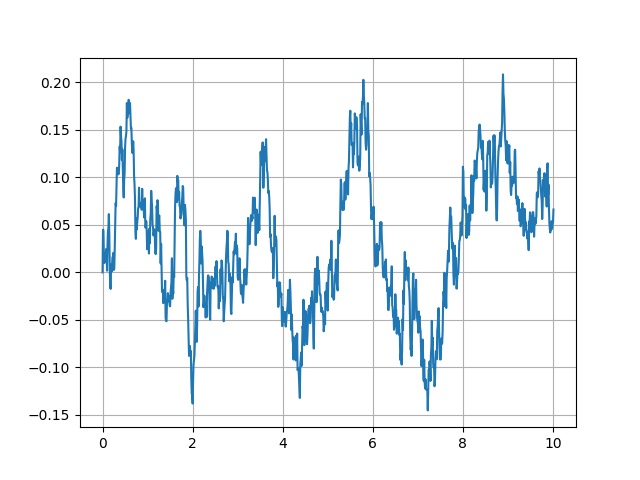
Figure 7 Score history for a single trajectory of the 1D double well model

Feel free to tweak the input parameters to see if you can trigger a transition ! We are all set to perform our first sampling run.

Sampling transitions

Let’s now use pyREVS to sample transition between the two wells. In particular, we are asking: what is the probability of a transition from well A (left) to well B (right) before a given time horizon \(T_a = 10\) ?

Similarly to the short script we wrote above to run a single trajectory, let assemble a small script to run the sampler (e.g. in sample_dw1D.py):

from pyrevs.sampler import build_sampler
from doublewell1D import doublewell1D

if __name__ == "__main__":
    # For convenience
    fmodel = doublewell1D

    # Initialize the algorithm object
    sampler = build_sampler(fmodel_t=fmodel)

    # Sample and report
    sampler.run()
    probability = sampler.database.get_event_probability()
    print(f"pyREVS transition probability: {probability}")

We also need to update the input file with additional parameters relative to the algorithm parameters. We will start with a Monte-Carlo sampling approach.

[sampler]
strategy = "montecarlo"

[montecarlo]
ntrajectories = 200
end_time = 10.0

[trajectory]
step_size = 0.01
targetscore = 0.95

[model]
epsilon = 0.04

[runner]
type = "asyncio"
nworkers=1

With above input parameters, the Monte-Carlo ensemble will contain 200 members. The model is assumed to have transitioned if the score function exceeds \(\xi_b = 0.95\). We will run using the asyncio runner, with a single worker during the initial ensemble generation. We have reduced the noise level to \(\epsilon = 0.04\).

Let’s now run the script:

python sample_dw1D.py

The algorithm should run for a few seconds, depending on your platform and how fast the model transitions. The default log level will report on the algorithm progress during the entire process, and reports a final summary of the form:

####################################################
# pyREVS v1.0.0                                    #
# Date: 2025-11-26 14:58:21.980592+00:00           #
# Model: doublewell1D                              #
# Sampling strategy: montecarlo                    #
####################################################
# Requested # of traj:                         200 #
# Number of 'Terminated' trajectories:         200 #
# Number of 'Converged' trajectories:            1 #
# Current total number of steps:            199792 #
####################################################

If you are lucky, maybe you will have one or two trajectories that transitioned and most likely none. Monte-Carlo sampling is included in pyREVS for testing purposes and can serve as a baseline for comparison with other sampling strategies, but it is very inefficient.

Let’s now switch to the TAMS algorithm. In the input file, update the strategy in the sampler section to ams (TAMS is a variant of AMS):

[sampler]
strategy = "ams"

and replace the montecarlo section with an ams section:

[ams]
ntrajectories = 50
nsplititer = 500
variant = "tams"
end_time = 10.0

With above input parameters, the TAMS ensemble will contain 50 members and the algorithm will proceed up to a total 500 selection/mutation events.

Let’s now run the script again:

python sample_dw1D.py

This time, the final summary should look something like:

####################################################
# pyREVS v1.0.0                                    #
# Date: 2025-11-26 14:58:21.980592+00:00           #
# Model: doublewell1D                              #
# Sampling strategy: ams                           #
####################################################
# Requested # of traj:                          50 #
# Number of 'Terminated' trajectories:          50 #
# Number of 'Converged' trajectories:           50 #
# Current total number of steps:            159868 #
####################################################

TAMS converged after 296 selection/mutation steps, time at which all 50 trajectories exceeded \(\xi_b\) within the 10 time units window. A total of 159868 model steps were taken and the transition probability estimate is \(\hat{P} = 2.46e^{-3}\). From a sampling perspective, it took 159868 model steps to obtain 50 trajectories that transitioned, where Monte-Carlo sampling required 199792 model steps for a single trajectory to transition. In order to compare the accuracy of the transition probability, we would need to run the TAMS algorithm several times.

Let’s update the sample script to extract more information from the sampling run:

from pyrevs.sampler import build_sampler
from doublewell1D import doublewell1D

if __name__ == "__main__":
    # For convenience
    fmodel = doublewell1D

    # Initialize the algorithm object
    sampler = build_sampler(fmodel_t=fmodel)

    # Sample and report
    sampler.run()
    probability = sampler.database.get_event_probability()
    print(f"pyREVS transition probability: {probability}")

    # Extract the envelope of the ensemble score function
    sampler.database.extension().plot_min_max_span("./doublewell1D_minmax.png")

and run the script again:

python sample_dw1D.py

The updated script above access the pyREVS database to show the history of the ensemble score functions span (the span of \(\mathcal{Q}_{tr}\)).

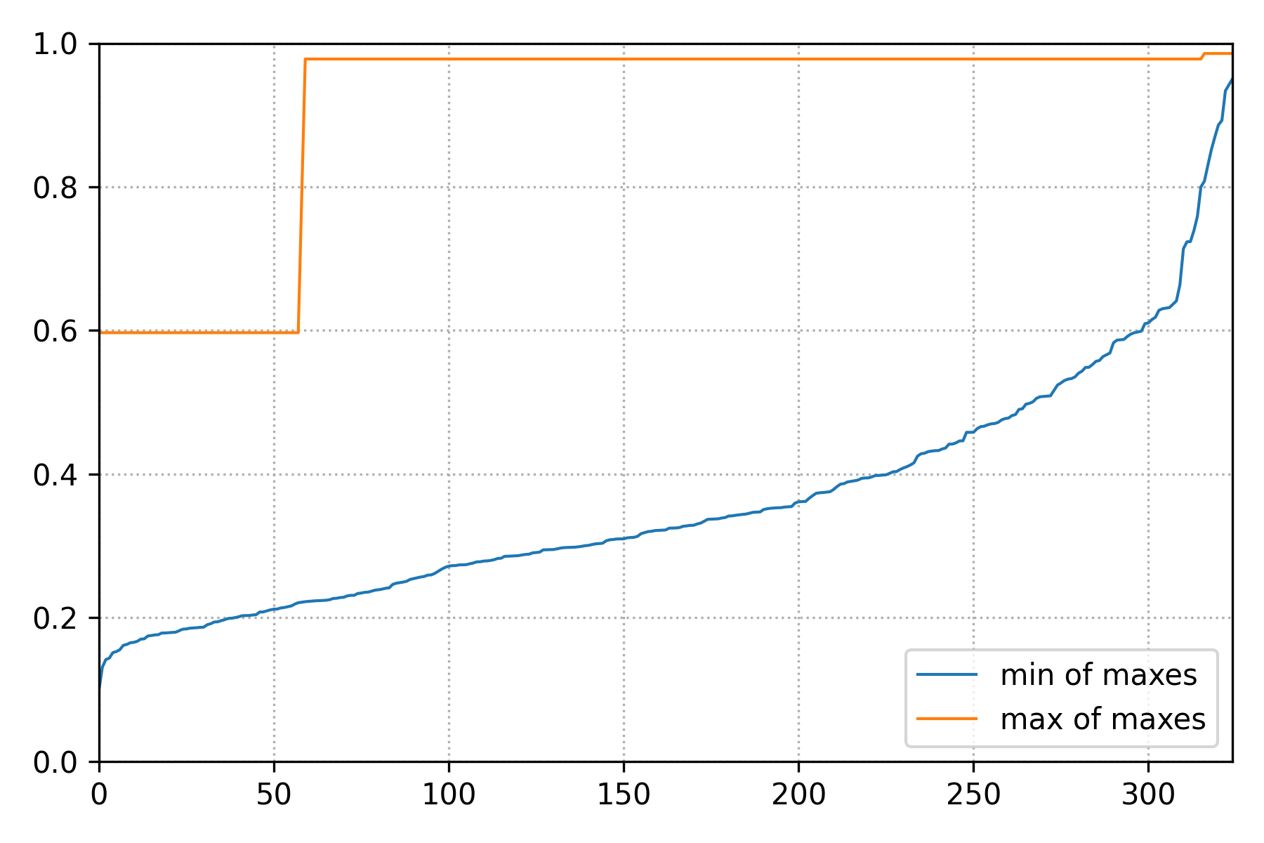
Figure 8 Span of \(\mathcal{Q}_{tr}\) over the course of the TAMS iterations.

We can this that in this high noise setting, one trajectory rapidly reaches \(\mathcal{B}\), but many more iterations are needed for the entire ensemble to transition.

Our final task will now focus on using AMS. With AMS, we are no longer interested in transition before a given time horizon, but rather: what is the probability that a model path exiting well A transitions to well B before returning to well A ?

To switch to sampling this particular probability, we do not need to update the forward model. You might have noticed that in the model initializer (__init__ function), we have set the initial condition close to well A, but not exactly at well A: i.e. x0 = -0.97 and not x0 = -1.0. As such our initial condition corresponds to a trajectory that is close to A, or exiting well A.

Let’s update the input file to enable AMS:

[ams]
ntrajectories = 50
nsplititer = 500
variant = "ams"
min_score = 0.01

With the above input parameters, the termination criterion is set such that return to well A corresponds to a score function value below 0.01. We can keep the ensemble envelope diagnostic in our sample script, but let’s also add another diagnostics allowing to monitor the ensemble during the AMS iterations:

[runtime]
plot_diagnostics = true

With the plot_diagnostics parameter set to True, pyREVS will plot the ensemble score functions at every AMS iteration. Let’s run the script again:

python sample_dw1D.py

The resulting transition probability is much lower than the one obtained with TAMS, which highlights the fact that the two methods are tracking very different quantities. Using the numerous images generated by pyREVS over the course of the algorithm enable to create an animation of the ensemble evolution:

Figure 9 Evolution of the AMS trajectories ensemble (\(N = 50\), \(l_j = 1\)) over the course the algorithm iterations.

You can compare the ensemble behavior with the one depicted in the Theory section.

This is all for this tutorial. We have covered the following points:

• Getting pyREVS

• Going from a pen-and-paper SDE to a practical implementation ready for pyREVS

• Testing the model on a single, isolated trajectory

• Running several sampling strategies, depending on the probability of interest.

To go further, modify the sample_dw1D.py script to run TAMS \(K\) times and provide a better estimate of the transition probability \(\overline{P}_K\), as well as its relative error. What happens when \(\epsilon\) is reduced? Can you trigger saving the pyREVS database to disk?

Bi-channel problem

In this tutorial, you will explore transitions in the bi-channel/triple wells, two-dimensional dynamical system. This system is regularly used for testing rare event algorithms, see for instance Brehier et al.. In contrast with the 1D double well tutorial, we will use the implementation already available in pyREVS examples and focus on using the algorithm to explore the system behavior.

Background

The bi-channel/triple well is a 2D overdamped diffusion process in which the potential landscape features two global minimum (at \((\pm 1.0, 0.0)\)) as well as a local minimum near \((0.0, 1.5)\). The global minima are connected by two channels: the upper channel through the local minima while the lower channel goes through the saddle point near \((0.0, -0.4)\). To take the upper channel, a trajectory will need to overcome two energy barriers to enter and exit the local minima, while the lower channel one feature a single barrier albeit of higher depth.

The potential as well as a system trajectory initiated near the left global minima \(\mathcal{A} = (x_A,y_A) = (-1,0)\) is presented in Fig. Figure 10.

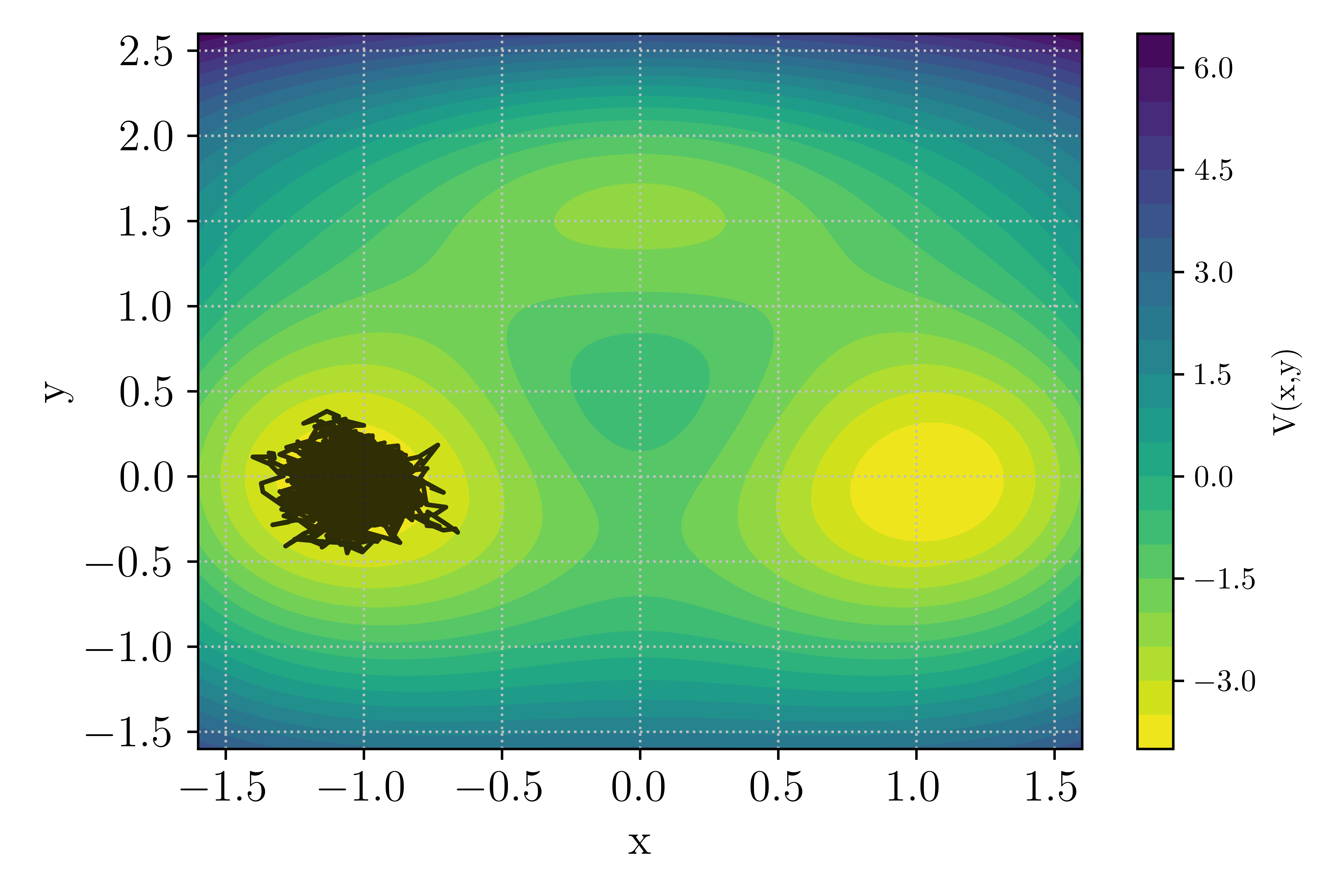
Figure 10 : Potential landscape of the bi-channel/triple well 2D case.

The noise level in this model is set by the inverse temperature parameter \(\beta\), with low values of \(\beta\) corresponding to a high noise level. At low noise levels, the upper channel is more likely as the two smaller energy barriers are easier to cross. In contrast, at high noise levels the shorter lower path becomes more likely as strong noise is able to push the system across the saddle point.

Getting set up

If you haven’t done so yet, let’s get pyREVS installed on your system. In order to have access to the example suite, you will need to install the package from sources.

git clone git@github.com:nlesc-eTAOC/pyREVS.git
cd pyREVS
pip install -e .
tams_check

The last line check that pyREVS is effectively installed and should return (with proper version numbers):

== pyREVS vX.Y.Z :: a rare-event finder tool ==

Move into the example folder

cd pyREVS/examples/BiChannel2D

The Forward Model

We will not have to modify the forward model in this tutorial, but it is still interesting to have a look at the content of the bichannel2d.py file. A quick check of the methods defined for this model reveals that all the required @abstractmethod from the pyREVS ABC are provided with a concrete implementations (see Tutorial on 1D double well for more details on this point).

In addition, a potential and drift are available to readily access the process parameters.

def _init_model(self, m_id: int, params: dict[str, typing.Any]) -> None:
def _advance(self, step: int, time: float, dt: float, noise: T_Noise, need_end_state: bool) -> float:
def potential(cls, x: npt.NDArray[np.number]) -> npt.NDArray[np.number]:
def drift(cls, x: npt.NDArray[np.number]) -> npt.NDArray[np.number]:
def get_current_state(self) -> T_State:
def set_current_state(self, state: T_State) -> None:
def score(self) -> float:
def make_noise(self) -> T_Noise:

The state is a Numpy array with two elements and the noise dimension is also \(m=2\). The model also uses an Euler-Murayama scheme to advance in time and the score function is the normalized distance to \(\mathcal{A}\):

\[\xi(X_t) = \frac{\Vert X_t - X_A \Vert_2}{\Vert X_B - X_A \Vert_2}\]

To test that the model is effectively available, you can reproduce Fig. Figure 10 by running the provided test script:

python test_bichannel.py

The script uses the Forward Model potential function to draw contours of \(V(x,y)\).

Running TAMS

Let’s now focus on running TAMS. As mentioned above, this case features two paths for transitioning from \(\mathcal{A} = X_A = (x_A,y_A) = (-1,0)\) to \(\mathcal{B} = X_B = (x_B,y_B) = (1,0)\). We will start with running TAMS using \(N=32\) and up to \(J=1000\) iteration. The time horizon is set to \(T_a = 20\) and the stopping criterion delimiting \(\mathcal{B}\) is \(\xi_b = 1.05\). All of these parameter can be set in the input.toml file (differs from default in the repository !):

[ams]
ntrajectories = 32
nsplititer = 1000
variant = "tams"
end_time = 20.0

[sampler]
strategy = "ams"

[runtime]
loglevel = "WARNING"

[trajectory]
step_size = 0.01
targetscore = 1.05

[model]
inv_temperature = 5.67

[runner]
type = "asyncio"
nworkers=1

Note that the log level here was decreased to WARNING in order to minimize standard output clutering when running TAMS multiple times. Let’s now look at the short script provided for running TAMS with the bi-channel model sample_bichannel.py:

import numpy as np
from bichannel2d import BiChannel2D
from bichannel2d import plot_in_landscape
from pyrevs.sampler import build_sampler

if __name__ == "__main__":
    # For convenience
    fmodel = BiChannel2D

    # Enable TAMS trajectory plots
    plot_ensemble = True

    # Number of consecutive sampling runs
    K = 10

    # Run the model several times
    for i in range(K):
        # Initialize the sampler
        sampler = build_sampler(fmodel_t=fmodel)

        # Sample and report
        try:
            sampler.run()
            probability = sampler.database.get_event_probability()
        except RuntimeError as e:
            print(e) # noqa: T201
            continue

        print(f"[{i}] : {probability}") # noqa: T201

        if plot_ensemble:
            plot_in_landscape(fmodel, sampler.database, i)

    print(f"Averaged transition P_K: {probabilities.mean()}, RE: {np.sqrt(probabilities.var()) / probabilities.mean()}")  # noqa : T201

As listed above, the script will perform \(K = 10\) consecutive sampling runs and report on the averaged transition probability \(P_K\) as well as the relative error. In addition, if the plot_ensemble is activated, a figure showing the TAMS trajectory ensemble in the potential landscape will be generated for each run. Let’s run the script:

python sample_bichannel.py

Depending on the platform you are using, it will take a few minutes to run.

Note

Some of the individual TAMS run might have terminated with: ` Splitting is stalling with all trajectories stuck at a score_max: 0.7399799334097721 ` This is an occurrence of extinction, a known issue of (T)AMS algorithms in which the ensemble collapse on a single ancestor trajectory and no significant progress is made through iterations until all trajectories have the same \(Q_{tr}\). This problem is more likely when using small ensemble or using a static score function in TAMS, as we do here.

At the value of the inverse temperature set in the input file \(\beta = 5.67\), transition through both channel can occurs with a significant probability such that out of the 10 runs, you should observe both upper and lower channel transition as depicted in the figure below.

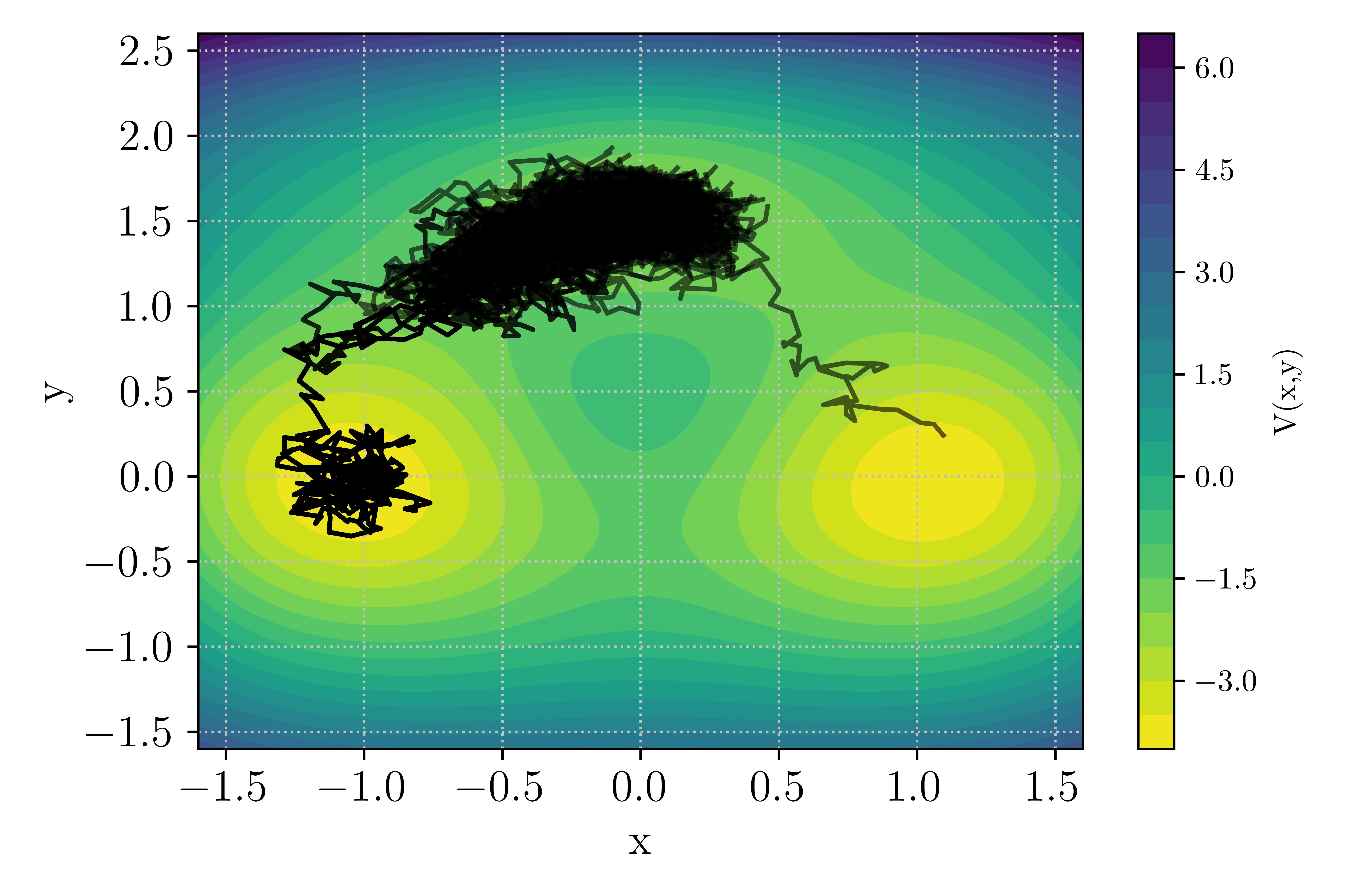
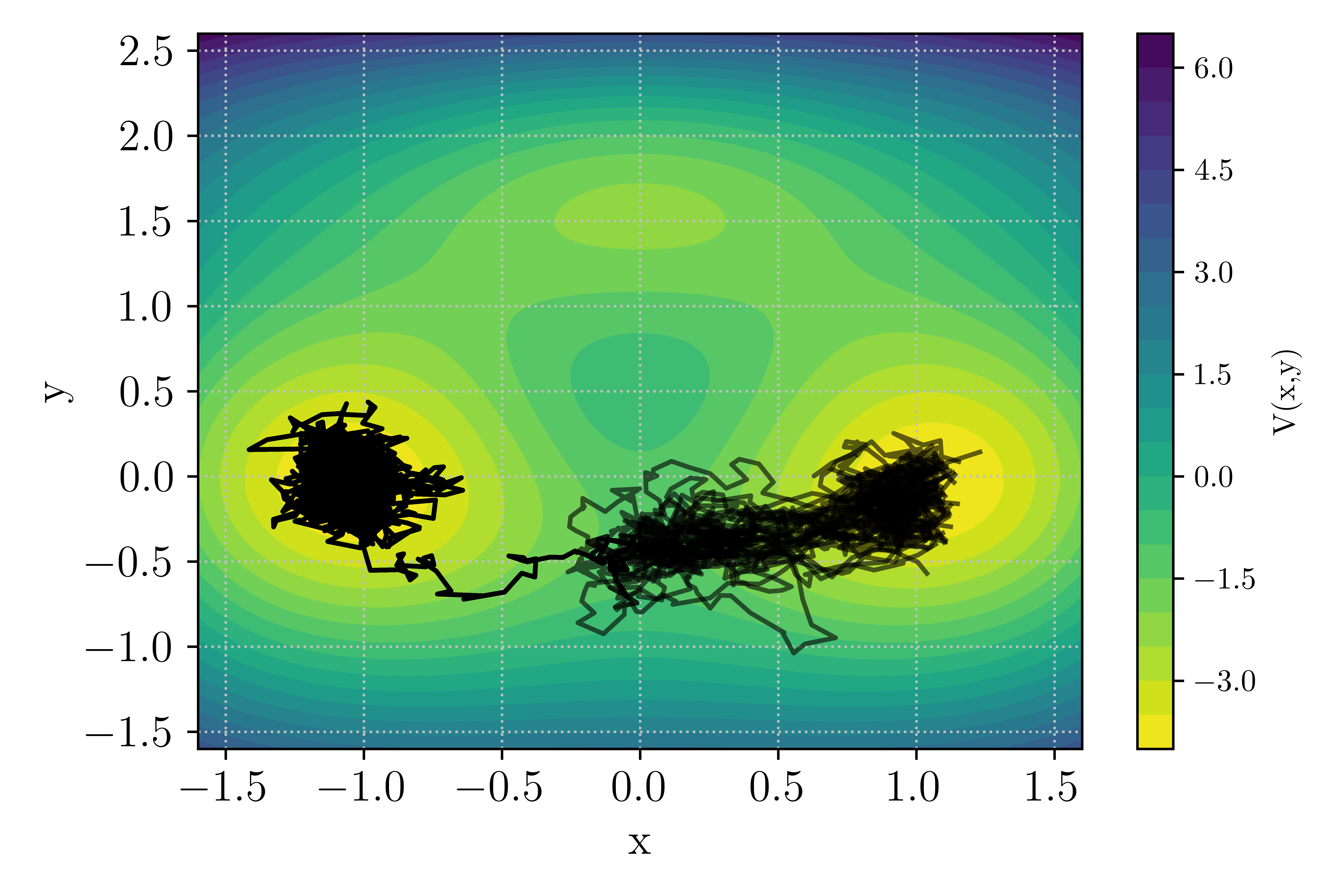
Figure 11 : Example of TAMS run with transition in the upper or lower channel

Let’s have a look at the behavior of the transition estimator \(P_K\) as \(K\) increases. This is similar to the experiment reported in Brehier et al., but we will limit the exercise to \(K = 200\). Running such an experiment would take significant time, beyond the scope of this tutorial. Instead, the probability of 200 TAMS runs are already available in the example folder and can be readily analyzed. Note that the data were generated using \(\beta = 6.67\) for which the transition probability is lower than in the earlier runs we performed here.

The data are stored in a Numpy file Pk_beta_6p67_K200.npy. We will write a small script to load the data and plot the evolution of \(P_K\) as \(K\) goes from 1 to 200. In a new Python file ((e.g. Pk_estimator.py):

import contextlib
import matplotlib.pyplot as plt
import numpy as np

if __name__ == "__main__":
    # Load the numpy data
    proba = np.load("./Pk_beta_6p67_K200.npy")

    # Initialize data containers for P_K
    # and the confidence interval
    pbar = np.zeros(proba.shape[0] - 1)
    pbar[0] = proba[0]
    pbar_ci = np.zeros(proba.shape[0] - 1)

    # Compute pbar and pbar_ci
    for k in range(1, proba.shape[0] - 1):
        pbar[k] = proba[:k].mean()
        pbar_ci[k] = 1.0 / np.sqrt(k) * np.sqrt(proba[:k].var())

    # Plot the results
    with contextlib.suppress(Exception):
        plt.rcParams.update({"text.usetex": True, "font.family": "serif"})
    plt.figure(figsize=(6, 4))
    plt.xticks(fontsize="x-large")
    plt.yticks(fontsize="x-large")
    plt.xlabel("$K$", fontsize="x-large")
    plt.ylabel("$P_K$", fontsize="x-large")
    plt.plot(np.linspace(1, proba.shape[0] - 1, proba.shape[0] - 1), pbar, color="r")
    plt.fill_between(
        np.linspace(1, proba.shape[0] - 1, proba.shape[0] - 1),
        pbar - pbar_ci,
        pbar + pbar_ci,
        color="r",
        alpha=0.2,
        linewidth=0.0,
    )
    plt.grid(linestyle=":", color="silver")
    plt.tight_layout()
    plt.show()

Running the script above in the bi-channel folder should produce the graph shown in Fig. Figure 12. Over the course of 200 runs, the estimator varies significantly and even with \(K = 200\) the value of \(P_K\) continues to change. Of interest is the shaded area, showing the 90% confidence interval, which gives an indication of the transition probability estimator quality.

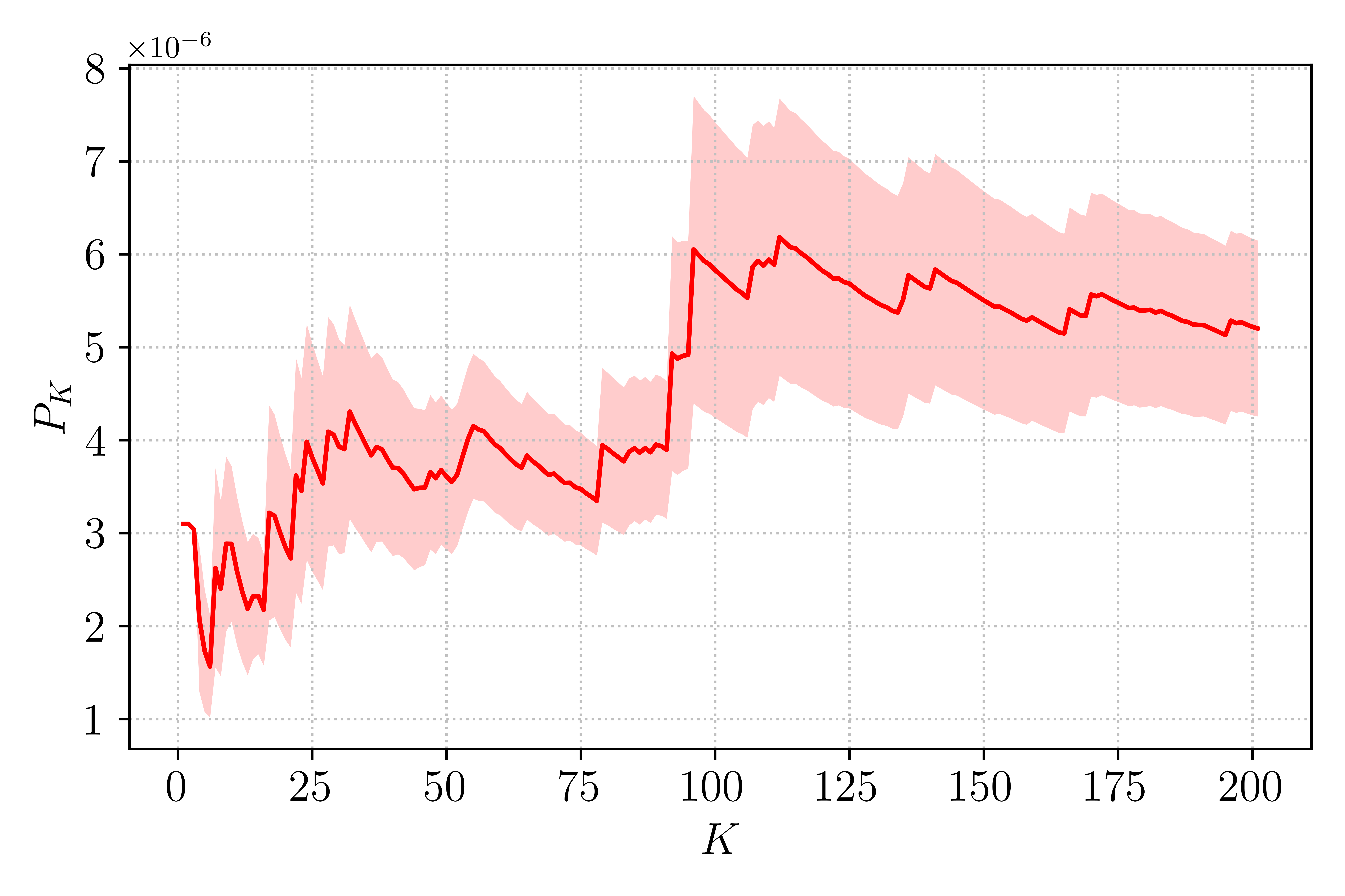
Figure 12 : Evolution of \(P_K\) with \(K\) repetitions of the TAMS algorithm.

Accessing the database

So far, we have performed multiple runs of pyREVS but have had limited access to the welth of data generated during the course of the algorithm. Looking back into the previous section, we have used the data to visualize the trajectory ensemble on the potential landscape. The pyREVS database object can be accessed during or after a sampling run using:

tdb = sampler.database

where sampler is an instance of the Sampler object. In the example script used above, the database object is send to the function constructing the plot: the plot_in_landscape function in bichannel2d.py. The few lines of code used to access the data in the database are reported below:

for t in tdb.traj_list():
    state_x = np.array([s[1][0] for s in t.get_state_list()])
    state_y = np.array([s[1][1] for s in t.get_state_list()])

Here we loop on the list of active trajectories tdb.traj_list(), i.e. the ensemble of \(N\) trajectories active at the current iteration of the algorithm. Note that when using a Monte-Carlo sampling strategy, only active trajectory are available. We then used Python list comprehension to go through the trajectory and extract a Numpy array of the system state components \(x\) and \(y\).

In our previous sampling runs, we could no longer access the database after exiting the script since the data was not saved to disk. Let’s now run one more time the algorithm, allowing to create a database on disk. To do so, let’s add the appropriate keyword to the input file input.toml:

[database]
path = "./db_tams_bichannel.tdb"

, update the sample_bichannel.py script to only run once by changing the value of \(K\):

# Number of consecutive sampling runs
K = 1

and run the script again:

python sample_bichannel.py

Note that saving the database to disk incurs an overhead, which is not negligeable for such a small model. Looking into your run folder should now show that a pyREVS database was saved:

ls -d db*
db_tams_bichannel.tdb

Let’s now put together a small script to load the database and access some of its data. In a new Python file (e.g. load_database.py):

from pyrevs.database import load_database
from pathlib import Path


if __name__ == "__main__":
    # Load the database from disk
    tdb = load_database(Path("./db_tams_bichannel.tdb"))
    tdb.load_data(load_archived_trajectories=True)

    # Show the ensemble scores at the last iteration
    tdb.plot_score_functions("./ScoreEnsemble.png")

    # Show the evolution of the ensemble span over
    # the course of TAMS iterations
    tdb.extension().plot_min_max_span("./ScoreMinMax.png")

    # Go through the active trajectories
    # and display the max score
    for t in tdb.traj_list():
        print(f"Trajectory {t.id()} final max score: {t.score_max()}")

    # Get the active trajectory list at initial iteration
    # and display the max score
    for t in tdb.extension().get_trajectory_active_at_k(0):
        print(f"Trajectory {t.id()} initial max score: {t.score_max()}")

The first line above instantiates the Database object, but only load metadata from disk. Only data such as the number of trajectories, the current index of the TAMS iteration and some trajectories metadata (did it converged, what is the maximum of the score function, …) are available. The load_data function effectively load the entire content of the trajectories in memory. By default only the active trajectory data are loaded, i.e. the trajectory at the end of the TAMS algorithm. By activating the load_archived_trajectories flag, we trigger loading the full list of trajectories including the ones discarded during the TAMS iterations. A couple of helper functions allow to asses the state of the ensemble by plotting the score functions as well as the evolution of the ensemble over the course of the iterations. One important point to note is the pyREVS database has a core component that contains the active and possibly archived trajectories. To access data from the ensemble, you can call tdb.<function>. For data associated with a specific sampling strategy (e.g. TAMS), you need to access the database extension with tdb.extensio().<function>. In the example above, we plot the trajectory ensemble score function through the core database function call tdb.plot_score_functions, but to plot the evolution of the ensemble over the course of the TAMS iterations, we need to use the extension tdb.extension().plot_min_max_span.

This is all for this tutorial. We have covered the following points:

• Exploring one of pyREVS built-in example

• Running TAMS multiple times in order to get a better transition probability estimator and uncertainty

• Accessing, saving and loading the pyREVS database

To go further, modify the change the value of the inverse temperature \(\beta\) parameter and see how that affect the probability of transitioning through the upper and lower channels, look at the Database and Trajectory APIs (database API) to extract more data from the database and get the most out of your sampling runs !

2D Boussinesq model

So far, the tutorials have been focused on fairly simple models for which pyREVS is practical, but also incurs a computational overhead that might not be justified compared to more simple implementation of sampling algorithms.

We will now turn our attention to a more complex model, with \(10^4\) degrees-of-freedom for which pyREVS is specifically designed for. The model is a stochastic partial differential equation (SPDE) described in Soons et al.. Two versions of this model are available in pyREVS examples and the present tutorial will focus on the C++ implementation examples/BoussinesqCpp in order to demonstrate how to couple pyREVS with an external software (as might be the case for many user of existing physics models). The interested reader can dig into the examples/Boussinesq to study the implementation of a Python-only version.

One final note to motivate the use of pyREVS: a \(10^4\) state requires about 80 kB of memory and considering a model trajectory consists of 4000 individual states, an active set of \(N=20\) trajectories requires about 6 GB of memory. This turns out to be only a fraction of the full memory requirements of TAMS as the total number of trajectories increases with the number of iterations, making it impossible to run TAMS on such a model without partially storing data to disk and sub-sampling the states (both native features of pyREVS).

Getting set up

If you haven’t done so yet, let’s get pyREVS installed on your system. In order to have access to the example suite, you will need to install the package from sources.

git clone git@github.com:nlesc-eTAOC/pyREVS.git
cd pyREVS
pip install -e .
tams_check

The last line check that pyREVS is effectively installed and should return (with proper version numbers):

== pyREVS vX.Y.Z :: a rare-event finder tool ==

Move into the example folder

cd pyREVS/examples/BoussinesqCpp

BoussinesqCpp Folder content

Before diving into the code, let’s first have a look at the content of the folder as many more files are involved compared to previous tutorials:

Boussinesq.cpp             # Implementation of physics model in C++
Boussinesq.h               # C++ model headers
Makefile                   # GNUmake file
Messaging.h                # Messaging library header, C++ side
OFFState.bin               # Model OFF state data, in binary format
OFFState.xmf               # Model OFF state data visualization (use Paraview)
ONState.bin                # Model ON state data, in binary format
ONState.xmf                # Model ON state data visualization (use Paraview)
README.md
__init__.py
boussinesq2d.py            # The forward model implementation
eigen_lapack_interf.h      # Eigen to LAPACK interface C++ header
input.toml                 # pyREVS input file
messaging.py               # Messaging library, Python side
sample_boussinesq2d.py     # Script for running sampler

There are three main components to this model:

• The model physics is encapsulated in a C++ program (Boussinesq.h, Boussinesq.cpp, eigen_lapack_interf.h)

• An inter-process communication (IPC) module with a C++ (Messaging.h) and a Python (messaging.py) side

• The pyREVS ABC concrete implementation for this model (boussinesq2d.py)

When coupling an external model to pyREVS, one should consider the possibility of maintaining the physics program continuously running in the background to avoid having to start and terminate the program repeatedly. In the present case, we implemented a simple IPC that enables running the C++ in the background all the time while controlling its flow from Python as pyREVS proceeds. This might not always be possible if you do not have access to the physics program source code.

Our aim here is not to dive too much into the C++ side, as the physics implementation is not particularly transferable to other cases, but to explore how to set up the ABC forward model implementation for an external program.

Let’s kick off this tutorial by compiling the physics program. Follow the instructions of the README.md file to obtain the external dependencies for this case (Eigen and LAPACK) and make sure you are able to compile the C++ program:

make
ls boussinesq.exe

BoussinesqCpp forward model

Let’s first look at the _init_model function in boussinesq2d.py to get a clear view of the model attributes:

self._m_id = m_id                             # The unique id of the model instance
self._M = params.get("size_M", 40)            # Number of grid point in latitude
self._N = params.get("size_N", 80)            # Number of grid point in depth
self._K = params.get("K", 7)                  # Number of Fourier modes for the stochastic forcing
self._eps = params.get("epsilon", 0.05)       # Variance of the Wiener noise process
self._exec = params.get("exec", None)         # The executable of the external physics program
self._exec_cmd = [                            # The command to start the external physics program
    self._exec,
    "-M",
    str(self._M),
    "-N",
    str(self._N),
    "-K",
    str(self._K),
    "--eps",
    str(self._eps),
    "--pipe_id",
    str(m_id),
]
self._proc = None                             # The id of the process of the external program
self._pipe = None                             # The IPC (named here pipe as it uses two-way pipes)
self._state = params.get("init_state", None)  # The model state

The model physical parameters are read from the input file (size_M, size_N, K, epsilon) and used to start the external program along with a path to its executable. The C++ program does not start at this point, but will be launched upon calling the advance function for the first time. In this model, the state is not directly the model state as an array of data but rather a path to a file on disk, generated/read by the external model. This has direct implication for the setter and getter function of the ABC: the set_current_state function must not only set the self._state variable on the Python side, but also communicate that information with the C++ program:

def set_current_state(self, state: T_State) -> None:
    """Set the model state.

    And transfer it to the C++ process if opened

    Args:
        state: the new state
    """
    self._state = state
    if not self._proc:
        return

    self._pipe.post_message(Message(MessageType.SETSTATE, data=state.encode("utf-8")))

    ret = self._pipe.get_message()
    if ret.mtype != MessageType.DONE:
        err_msg = "Unable to set the state of the C++ code"
        _logger.error(err_msg)
        raise RuntimeError

If we now take a closer look at the advance function, there are a few notable things to notice:

def _advance(self, _step: int, _time: float, dt: float, noise: Any, need_end_state: bool) -> float:
    """Advance the model.

    Args:
        step: the current step counter
        time: the starting time of the advance call
        dt: the time step size over which to advance
        noise: the noise to be used in the model step
        need_end_state: whether the step end state is needed

    Return:
        Some model will not do exactly dt (e.g. sub-stepping) return the actual dt
    """
    if not self._proc:
        # Initialize the C++ process and the twoway pipe
        self._proc = subprocess.Popen(self._exec_cmd)

        self._pipe = TwoWayPipe(str(self._m_id))
        self._pipe.open()

        # Send the workdir
        self._pipe.post_message(Message(MessageType.SETWORKDIR, data=self._workdir.as_posix().encode("utf-8")))

        # Set the initial state
        self.set_current_state(self._state)

    if need_end_state:
        self._pipe.post_message(trigger_save_msg)

    self._pipe.post_message(Message(MessageType.ONESTOCHSTEP, data=noise.tobytes()))
    ret = self._pipe.get_message()
    if ret.mtype != MessageType.DONE:
        err_msg = "Unable to access the score from the C++ code"
        _logger.error(err_msg)
        raise RuntimeError

    self._score = struct.unpack("d", ret.data)[0]

    if need_end_state:
        self._state = self.get_last_statefile()
    else:
        self._state = None

    return dt

• Upon the first call to the advance function, the C++ program is started using Python subprocess. At the same time, the IPC two-way pipe is initialized and the initial condition communicated to the external program.

• pyREVS’s trajectory API allows to downsample the state stored in the trajectory and the advance function need_end_state argument is set to True when the algorithm expects a state. This is also transferred to the C++ program before effectively advancing the model. Depending on how your model handles IO, you can use this parameter to make sure a checkpoint file is generated (or possibly suppress a checkpoint file if your model always produces IO but it is not needed)

The noise increment for the model’s stochastic forcing is still generated on the Python side and communicated to the external C++ program when performing a model time step. Additionally, the Python ABC does not have access to the C++ program state variables (i.e. the physical field of temperature, salinity, …) and must query the model to get the score function (transferring entire variable fields to Python would slow the model significantly).

One last function worth noting is _clear_model:

def _clear_model(self) -> None:
    if self._proc:
        self._pipe.post_message(exit_msg)
        self._proc.wait()
        self._proc = None
        self._pipe.close()
        self._pipe = None

This function is part of pyREVS forward model ABC but does not need to be overwritten by a concrete implementation. It is always called upon completing a trajectory (i.e. reaching the score function target value or an other termination condition) and in the current model, it terminates the external C++ program.

Running pyREVS locally

We will now sample the Boussinesq model transition with TAMS. This model is significantly more computationally expensive that the other models used in previous tutorials, but it still only takes a few dozens minutes to perform a sampling run on a laptop.

Let’s review the content of the input file input.toml:

[sampler]
strategy = "ams"

[ams]
ntrajectories = 20
nsplititer = 200
variant = "tams"
end_time = 20.0

[runtime]
loglevel = "INFO"
plot_diagnostics = true

The number of ensemble members is set to \(N=20\) and the maximum of iteration set to \(J = 200\). We enable plot diagnostic to True is order to visualize the evolution of the ensemble during the course of the iterations, as depicted in the last graph of the Theory Section.

[trajectory]
step_size = 0.005
targetscore = 0.95
sparse_freq = 10

The time horizon is set to \(T_a = 20\) time units and the step size 0.005. The target score function defining the model AMOC collapsed state is \(\xi_b = 0.95\). Finally, only one state every 10 steps will be requested (i.e. the advance function argument need_end_state will be False 9 out of 10 calls. This reduce by an order of magnitude the disk space requirements. Note that this parameter is a disk space versus compute trade-off, as sparser trajectory will require to recompute some model steps during the cloning/branching step of the algorithm.

[model]
exec = "./boussinesq.exe"
init_state = "./ONState.bin"
size_M = 40
size_N = 80
epsilon = 0.05
K = 7

The model parameters are parsed in the model _init_model function and control the size of computational model as well as stochastic forcing shape and intensity. The initial condition is set to be the AMOC ON state. Note that the noise level here is fairly high \(\epsilon = 0.05\), such that the transition is not so rare in order to limit the compute time.

[runner]
type = "dask"
nworkers=2

When running the model locally, both asyncio and dask runner are valid options. Here we use Dask by default, spawning two workers during the initial ensemble generation and two workers during the TAMS iterations. The later parameter effectively means that at least the two trajectories with the lowest values of the maximum score function will be discarded and new trajectory cloned/branched at each TAMS iterations.

[database]
path = "2DBoussinesqCpp.tdb"

Running this model always requires creating a database on disk to store the external model data.

As with previous Tutorials, there a short script in the example folder to launch the sampling run:

python sample_boussinesq2d.py

For the sake of keeping this tutorial short, only a single sampling run is required.

The standard output should look something like:

[INFO] 2025-12-04 22:46:02,769 -
            ####################################################
            # pyREVS v1.0.0                                    #
            # Date: 2025-12-04 21:46:02.752567+00:00           #
            # Model: 2DBoussinesqModelCpp                      #
            # Strategy: ams                                    #
            ####################################################
            # Requested # of traj:                          20 #
            # Number of 'Terminated' trajectories:           0 #
            # Number of 'Converged' trajectories:            0 #
            # Current total number of steps:                 0 #
            ####################################################

[INFO] 2025-12-04 22:46:02,785 - Computing 2DBoussinesqModelCpp rare event probability using TAMS
[INFO] 2025-12-04 22:46:02,785 - Creating the initial ensemble of 20 trajectories
[INFO] 2025-12-04 22:46:03,292 - Advancing traj000002_0000 [time left: 86399.487147]
[INFO] 2025-12-04 22:46:03,293 - Advancing traj000003_0000 [time left: 86399.486938]
[INFO] 2025-12-04 22:46:28,092 - Advancing traj000018_0000 [time left: 86374.679952]
[INFO] 2025-12-04 22:46:28,120 - Advancing traj000006_0000 [time left: 86374.651914]
...
[INFO] 2025-12-04 22:50:49,663 - Advancing traj000010_0000 [time left: 86113.108818]
[INFO] 2025-12-04 22:51:14,384 - Advancing traj000012_0000 [time left: 86088.387617]
[INFO] 2025-12-04 22:51:14,437 - Advancing traj000000_0000 [time left: 86088.334118]
[INFO] 2025-12-04 22:51:39,418 - Run time: 336.648924 s
[INFO] 2025-12-04 22:51:39,418 - Using multi-level splitting to get the probability
[INFO] 2025-12-04 22:51:39,992 - Starting TAMS iter. 0 with 2 workers
[INFO] 2025-12-04 22:51:40,595 - Restarting [19] from traj000003_0000 [time left: 86062.184477]
[INFO] 2025-12-04 22:51:40,597 - Restarting [4] from traj000001_0000 [time left: 86062.183612]
[INFO] 2025-12-04 22:52:02,934 - Starting TAMS iter. 2 with 2 workers
[INFO] 2025-12-04 22:52:03,365 - Restarting [10] from traj000019_0001 [time left: 86039.406361]
[INFO] 2025-12-04 22:52:03,383 - Restarting [2] from traj000017_0000 [time left: 86039.388611]
[INFO] 2025-12-04 22:52:23,398 - Starting TAMS iter. 4 with 2 workers
...
[INFO] 2025-12-04 22:59:55,533 - Starting TAMS iter. 102 with 2 workers
[INFO] 2025-12-04 22:59:55,848 - Restarting [8] from traj000016_0008 [time left: 85566.924079]
[INFO] 2025-12-04 22:59:55,879 - Restarting [7] from traj000000_0003 [time left: 85566.892251]
[INFO] 2025-12-04 22:59:57,955 - Starting TAMS iter. 104 with 2 workers
[INFO] 2025-12-04 22:59:58,134 - All trajectories converged after 104 splitting iterations
[INFO] 2025-12-04 22:59:58,317 - Run time: 835.547348 s
[INFO] 2025-12-04 23:00:02,499 - 104 archived trajectories loaded
[INFO] 2025-12-04 23:00:02,521 -
            ####################################################
            # TAMS v0.0.6             trajectory database      #
            # Date: 2025-12-04 21:46:02.752567+00:00           #
            # Model: 2DBoussinesqModelCpp                      #
            ####################################################
            # Requested # of traj:                          20 #
            # Requested # of splitting iter:               500 #
            # Number of 'Ended' trajectories:               20 #
            # Number of 'Converged' trajectories:           20 #
            # Current splitting iter counter:              106 #
            # Current total number of steps:            183619 #
            # Transition probability:    0.0037570973859534823 #
            ####################################################

Since diagnostic is set to True, a series of images Score_k0****.png showing the ensemble at each iterations (every two cloning/branching events) is generated.

Running pyREVS on a Slurm cluster

In the event you have access to an HPC cluster, we will now update the input file to run pyREVS on a Slurm cluster.

[ams]
walltime = 7100

[runner.dask]
backend = "slurm"
worker_walltime = "2:00:00"
queue = "genoa"
ntasks_per_job = 1
job_prologue = ['module load Python', 'conda activate pyREVS']

The default backend of the dask runner is local, by setting it to slurm Dask will submit the workers as Slurm jobs. The job wall time will be set to 2 hours and be submitted to the genoa partition. The algorithm walltime must thus be updated to not exceed the job wall time. The strings listed in the job_prologue will be executed before starting the worker and can be used to setup your environment.

If your cluster allows it, can launch the sampling script from the login node (very to no compute is done by the main process in pyREVS), otherwise you will have to launch the sampling script from a Slurm batch script.

This is all for this tutorial. We have covered the following points:

• Interfacing an external program with pyREVS

• Triggering diagnostics while running TAMS sampling

• Using multiple workers and running pyREVS on a Slurm cluster

To go further, interested users can change the model noise parameters or repeat the experiment multiple times. Additionally, the Python version of the Boussinesq model has several custom features and comparing the two implementations could be a good source of information for developing your own model.